PyTorch로 전문가 혼합(MoE) 모델 학습 확장하기

최근 1년간 전문가 혼합(MoE, Mixture-of-Experts) 모델들의 인기가 급증했습니다. 이러한 인기는 DBRX, Mixtral, DeepSeek를 비롯하여 다양하고 강력한 오픈소스 모델들로부터 비롯된 것입니다. Databricks에서는 PyTorch 팀과 협력하여 MoE 모델의 학습을 확장했습니다. 이번 글에서는 PyTorch Distributed 및 PyTorch로 구현한 효율적인 오픈소스 MoE 구현체인 MegaBlocks를 사용하여 학습을 3천개 이상의 GPU들로 확장하는 방법에 대해 이야기해보겠습니다.

Over the past year, Mixture of Experts (MoE) models have surged in popularity, fueled by powerful open-source models like DBRX, Mixtral, DeepSeek, and many more. At Databricks, we’ve worked closely with the PyTorch team to scale training of MoE models. In this blog post, we’ll talk about how we scale to over three thousand GPUs using PyTorch Distributed and MegaBlocks, an efficient open-source MoE implementation in PyTorch.

전문가 혼합(MoE)이 무엇인가요? / What is a MoE?

전문가 혼합(MoE, Mixture-of-Experts) 모델은 여러 전문가 네트워크들을 사용하여 예측을 수행하는 모델 구조입니다. 게이팅(gating) 네트워크는 전문가 네트워크들의 출력을 라우팅하고 결합하는데 사용하며, 각 전문가가 서로 다른 토큰들의 분포(specialized distribution of tokens)로 학습되도록 합니다. 트랜스포머 기반의 대규모 언어 모델(LLM, Large Language Model)은 일반적으로 임베딩 레이어 뒤에 여러 개의 트랜스포머 블록들로 구성됩니다. (그림 1, 제일 왼쪽 A) 각 트랜스포머 블록에는 어텐션 블록(attention block)과 덴스 피드 포워드 네트워크(dense feed forward network)가 포함되어 있습니다. (그림 1, 왼쪽 두번째 B) 이러한 트랜스포머 블록들은 하나의 블록의 출력이 다음 블록의 입력으로 이어지도록 쌓여 있습니다. 최종 출력은 완전 연결된 레이어(fully connected layer)와 소프트맥스(softmax)를 거쳐 다음에 출력할 토큰에 대한 확률을 얻습니다.

A MoE model is a model architecture that uses multiple expert networks to make predictions. A gating network is used to route and combine the outputs of experts, ensuring each expert is trained on a different, specialized distribution of tokens. The architecture of a transformer-based large language model typically consists of an embedding layer that leads into multiple transformer blocks (Figure 1, Subfigure A). Each transformer block contains an attention block and a dense feed forward network (Figure 1, Subfigure B). These transformer blocks are stacked such that the output of one transformer block leads to the input of the next block. The final output goes through a fully connected layer and softmax to obtain probabilities for the next token to output.

LLM에 MoE를 적용할 때는, 덴스 피드 포워드 레이어(dense feed forward layer)가 MoE 레이어로 대체됩니다. MoE 레이어는 게이팅 네트워크와 여러 전문가들로 구성됩니다. (그림 1, 오른쪽 D) 게이팅 네트워크는 일반적으로 선형 피드 포워드 네트워크(linear feed forward network)로, 각 토큰을 받아 어떤 토큰이 어떤 전문가로 라우팅되어야 하는지 결정하도록 하는 가중치 세트(set of weights)를 생성합니다. 전문가 네트워크들 자체도 일반적으로 피드 포워드 네트워크로 구현합니다. 학습 중에는 게이팅 네트워크는 입력을 전문가들에게 할당하여, 모델이 특화되고 성능이 향상되도록 합니다. 이후, 라우터 출력을 전문가 출력을 더하여(weigh) MoE 레이어의 최종 출력으로 제공합니다.

When using a MoE in LLMs, the dense feed forward layer is replaced by a MoE layer which consists of a gating network and a number of experts (Figure 1, Subfigure D). The gating network, typically a linear feed forward network, takes in each token and produces a set of weights that determine which tokens are routed to which experts. The experts themselves are typically implemented as a feed forward network as well. During training, the gating network adapts to assign inputs to the experts, enabling the model to specialize and improve its performance. The router outputs are then used to weigh expert outputs to give the final output of the MoE layer.

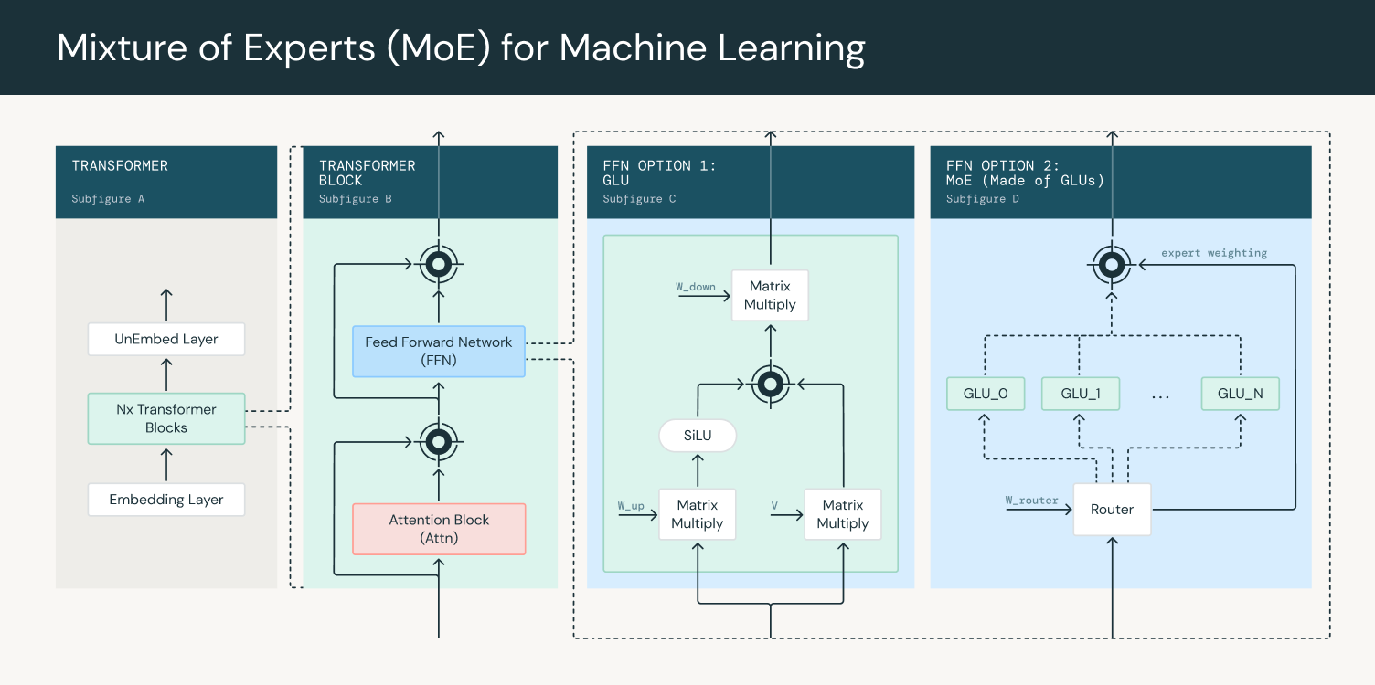
그림 1: 트랜스포머 블록에서 전문가 혼합(MoE) 사용하기 / Figure 1: Using Mixture of Experts in a transformer block

더 큰 밀집된 모델(dense model)들에 비해, MoE 모델은 주어진 연산 한도(compute budget)로 더 효율적으로 학습할 수 있습니다. 이는 게이팅 네트워크가 토큰을 전문가들 중 일부에게만 보내어 연산 부하를 줄이기 때문입니다. 결과적으로, 모델의 용량(= 전체 매개변수의 수)을 늘리면서도 이에 비례하여 연산 요구 사항(computational requirements)을 늘리지 않아도 됩니다. 추론 시에는 전문가들 중 일부만 사용하므로 MoE는 더 큰 밀집된 모델(dense model)에 비해 더 빠르게 추론을 수행할 수 있습니다. 그러나, 메모리에는 사용 중인 전문가들만이 아니라 전체 모델을 불러와야(loaded) 합니다.

Compared to dense models, MoEs provide more efficient training for a given compute budget. This is because the gating network only sends tokens to a subset of experts, reducing the computational load. As a result, the capacity of a model (its total number of parameters) can be increased without proportionally increasing the computational requirements. During inference, only some of the experts are used, so a MoE is able to perform faster inference than a dense model. However, the entire model needs to be loaded in memory, not just the experts being used.

MoE의 희소성(sparsity)은 특정 토큰이 일부 전문가들에게만 라우팅되도록 하여 연산 효율을 높여줍니다. 전문가의 수와 전문가를 선택하는 방법은 게이팅 네트워크의 구현에 따라 다르지만, 상위 k개(top-k)가 일반적인 방법입니다. 게이팅 네트워크는 먼저 각 전문가들에 대한 확률 값을 예측한 다음, 상위 k개의 전문가들(top k experts)에게 토큰을 전달(route)하여 출력을 얻습니다. 하지만, 모든 토큰들이 항상 동일한 일부 전문가들에게만 전달되면, 학습이 비효율적으로 되고 다른 전문가들은 학습이 잘 되지 않게 됩니다. 이러한 문제를 완화하기 위해 모든 전문가들에게 고르게(even) 라우팅되도록 하는 로드 밸런싱 손실(load balancing loss)이 도입되었습니다.

The sparsity in MoEs that allows for greater computational efficiency comes from the fact that a particular token will only be routed to a subset of experts. The number of experts and how experts are chosen depends on the implementation of the gating network, but a common method is top k. The gating network first predicts a probability value for each expert, then routes the token to the top k experts to obtain the output. However, if all tokens always go to the same subset of experts, training becomes inefficient and the other experts end up undertrained. To alleviate this problem, a load balancing loss is introduced that encourages even routing to all experts.

전문가의 수와 상위 k개의 전문가를 고르는 것은 MoE 모델 설계 시의 중요한 요소입니다. 전문가의 수가 많을수록 연산 비용을 늘리지 않으면서도 더 큰 모델로 확장할 수 있습니다. 이는 모델이 더 많은 학습을 할 수 있는 능력(capacity)을 갖춤을 뜻하지만, 일정 수준 이상으로 전문가의 수를 늘리면 성능 향상이 줄어드는(diminish) 경향이 있습니다. 전체 모델을 메모리에 불러와야 하므로 몇 개의 전문가를 선택할지는 모델 서빙 시의 추론 비용과 균형을 맞춰야 합니다. 상위 k개(top-k)를 선택할 때도 마찬가지로, 학습 중에 더 작은 k개를 선택하면 행렬 곱 연산(matrix multiplication)을 적게 수행하게 되어, 통신 비용이 큰 경우 연산 자원이 남게(leaving free computation on the table) 됩니다. 하지만 더 큰 k개를 선택하면 추론 속도가 일반적으로 느려지게 됩니다.

The number of experts and choosing the top k experts is an important factor in designing MoEs. A higher number of experts allows scaling up to larger models without increasing computational cost. This means that the model has a higher capacity for learning, however, past a certain point the performance gains tend to diminish. The number of experts chosen needs to be balanced with the inference costs of serving the model since the entire model needs to be loaded in memory. Similarly, when choosing top k, a lower top k during training results in smaller matrix multiplications, leaving free computation on the table if communication costs are large enough. During inference, however, a higher top k generally leads to slower inference speed.

메가블록 / MegaBlocks

MegaBlocks은 희소 행렬 곱(sparse matrix multiplication)을 사용하여 토큰 할당이 불균형(uneven)하더라도 전문가 출력을 병렬로 연산하는 효율적인 MoE 구현체입니다. MegaBlocks는 GPU 커널을 사용하는 동안 토큰을 버리지 않으므로(avoid dropping tokens) 효율적인 학습을 유지하는 Dropless MoE를 구현합니다. MegaBlocks 이전에는 연산 시 토큰을 버리거나 패딩(padding)에 연산 자원과 메모리를 낭비하는 등, 모델 품질(model quality)과 하드웨어 효율성(hardware efficiency) 사이에서 절충점(trade-offs)을 찾아야 하는 동적 라우팅 공식(dynamic routing dormulation)을 사용했습니다. 전문가 네트워크들은 다양한 수의 토큰들(variable number of tokens)을 받을 수 있으며, 전문가 연산(expert computation)은 블록 희소 행렬 곱(block sparse matrix multiplication)을 사용하여 효율적으로 수행할 수 있습니다. 우리는 LLM Foundry에 MegaBlocks를 통합(integrate)하여 MoE 학습을 수천개의 GPU로 확장할 수 있도록 했습니다.

MegaBlocks is an efficient MoE implementation that uses sparse matrix multiplication to compute expert outputs in parallel despite uneven token assignment. MegaBlocks implements a dropless MoE that avoids dropping tokens while using GPU kernels that maintain efficient training. Prior to MegaBlocks, dynamic routing formulations forced a tradeoff between model quality and hardware efficiency. Previously, users had to either drop tokens from computation or waste computation and memory on padding. Experts can receive a variable number of tokens and the expert computation can be performed efficiently using block sparse matrix multiplication. We’ve integrated MegaBlocks into LLM Foundry to enable scaling MoE training to thousands of GPUs.

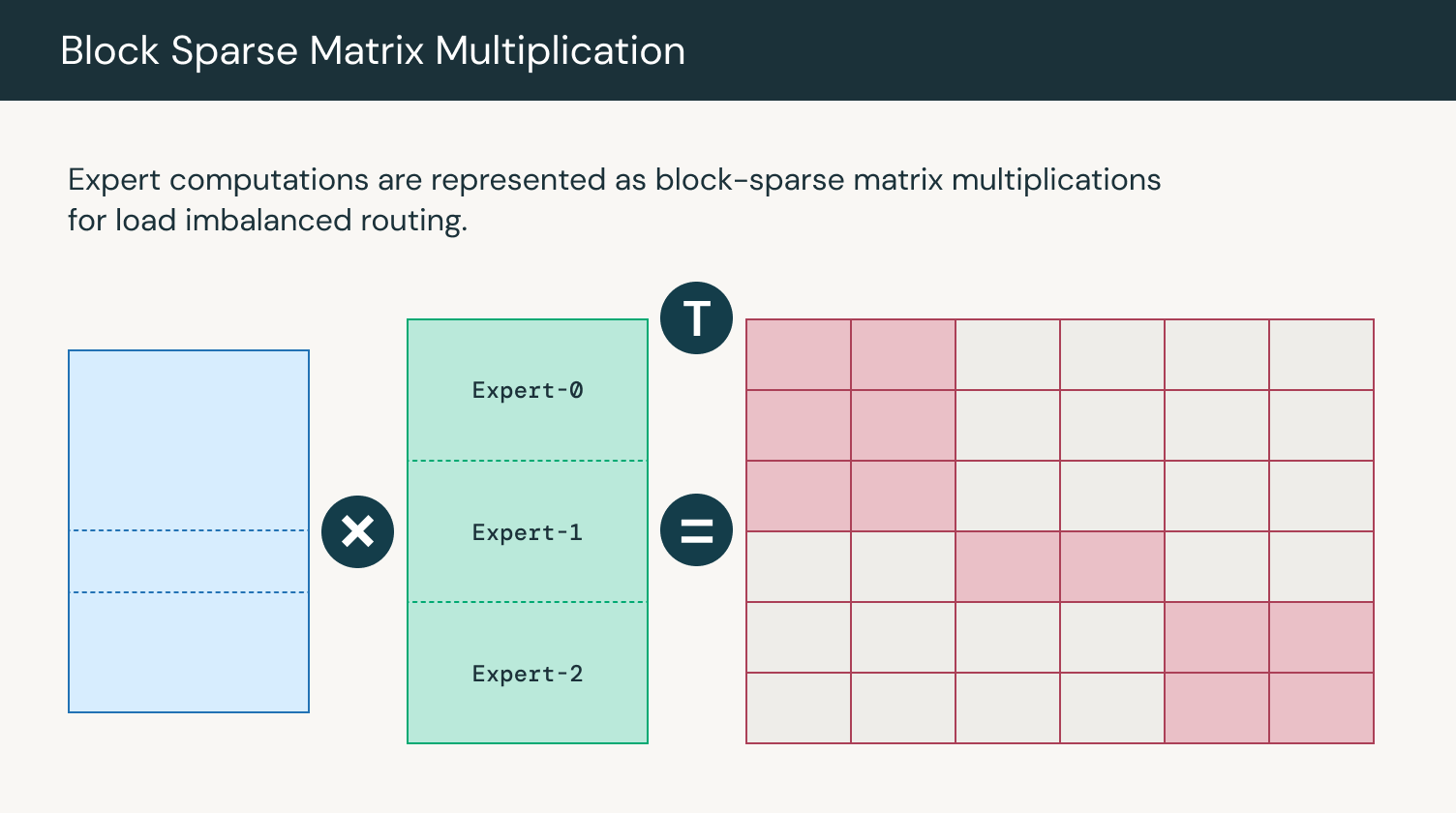
그림 2: 전문가 연산 시의 행렬 곱 연산 / Figure 2: Matrix multiplication for expert computations

전문가 병렬화 / Expert Parallelism

모델이 더 큰 크기로 확장되어 하나의 GPU에 올라가지 않는다면, 더 고급 형태의 병렬 처리(advanced forms of parallelism)가 필요합니다. 전문가 병렬화(Expert Parallelism)는 모델 병렬화(Model Parallelism)의 일종으로, 성능 향상을 위해 서로 다른 GPU에 서로 다른 전문가를 배치하는 형태입니다. 전문가 네트워크의 가중치들을 모든 GPU들 간에 공유(communicate)하는 대신, 토큰들이 각 전문가를 포함하고 있는 장치로 전송됩니다. 가중치 대신 데이터를 이동함으로써, 여러 기기들(multiple machines)에서 단일 전문가 네트워크를 위한 데이터를 집계(aggregate)할 수 있습니다. 라우터(router)는 입력 시퀀스(input sequence)에서 어떤 토큰을 어떠한 전문가에게 보낼지를 결정합니다. 이는 일반적으로 각 토큰-전문가 쌍(token-expert pair)에서 게이팅 점수(gating score)를 계산한 다음, 각 토큰을 최고 점수를 받은 전문가쪽으로 전달(route)하는 식으로 이뤄집니다. 토큰별 전문가 할당(token-to-expert assignment)이 결정되고 나면, 전체-대-전체(all-to-all) 통신 단계를 수행하여 해당 전문가를 호스팅하는 장치로 토큰을 전송합니다. 이 단계에는 각 디바이스들이 해당 장치의 전문가에게 할당된 토큰을 받는 동시에 다른 디바이스의 전문가에게 할당된 토큰을 보내는 과정이 포함됩니다.

As models scale to larger sizes and fail to fit on a single GPU, we require more advanced forms of parallelism. Expert parallelism is a form of model parallelism where we place different experts on different GPUs for better performance. Instead of expert weights being communicated across all GPUs, tokens are sent to the device that contains the expert. By moving data instead of weights, we can aggregate data across multiple machines for a single expert. The router determines which tokens from the input sequence should be sent to which experts. This is typically done by computing a gating score for each token-expert pair, and then routing each token to the top-scoring experts. Once the token-to-expert assignments are determined, an all-to-all communication step is performed to dispatch the tokens to the devices hosting the relevant experts. This involves each device sending the tokens assigned to experts on other devices, while receiving tokens assigned to its local experts.

전문가 병렬화의 주요 장점은 여러 개의 작은 행렬 곱셈(matrix multiplication) 대신, 몇 개의 더 큰 행렬 곱셈을 처리할 수 있다는 것입니다. 각 GPU는 전문가의 일부만을 가지고 있기 때문에, 해당 전문가에 대한 연산만 수행하면 됩니다. 따라서 여러 GPU들 간의 토큰을 집계하면 각 행렬의 크기도 비례해서 커집니다. GPU는 대규모 병렬 연산에 최적화되어 있으므로, 대규모 작업일수록 그러한 기능들을 더 잘 활용할 수 있어 활용도(utilization)와 효율성(efficiency)이 높아집니다. 더 큰 행렬 곱셈의 이점에 대한 보다 자세한 설명은 여기에서 확인할 수 있습니다. 연산이 완료되고 나면 전문가의 출력을 원래 장치로 보내기 위해 다시 전체-대-전체(all-to-all) 통신 단계가 수행됩니다.

The key advantage of expert parallelism is processing a few, larger matrix multiplications instead of several small matrix multiplications. As each GPU only has a subset of experts, it only has to do computation for those experts. Correspondly, as we aggregate tokens across multiple GPUs, the size of each matrix is proportionally larger. As GPUs are optimized for large-scale parallel computations, larger operations can better exploit their capabilities, leading to higher utilization and efficiency. A more in depth explanation of the benefits of larger matrix multiplications can be found here. Once the computation is complete, another all-to-all communication step is performed to send the expert outputs back to their original devices.

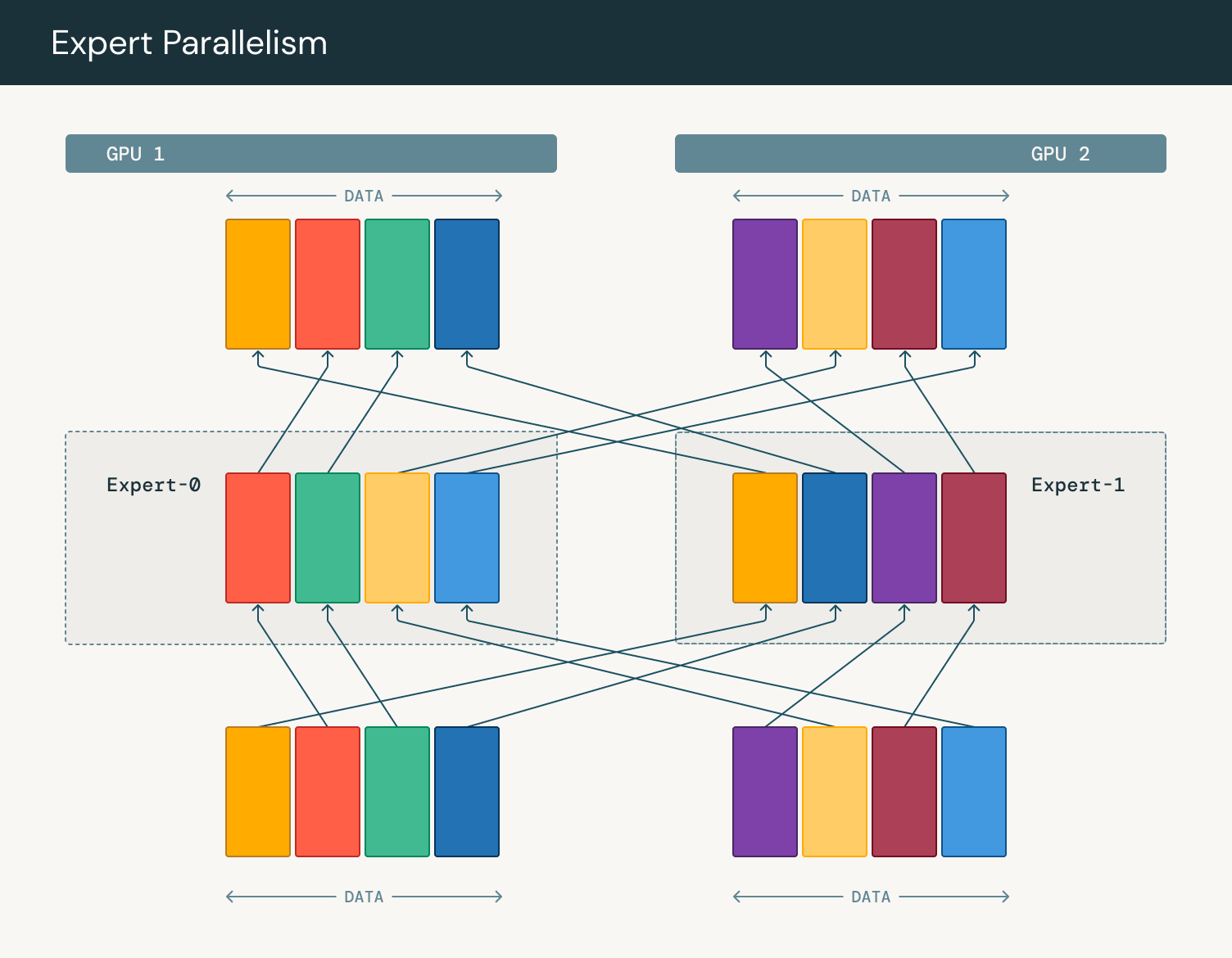
그림 3: 전문가 병렬화에서의 토큰 라우팅 / Figure 3: Token routing in expert parallelism

우리는 텐서가 어떻게 샤딩(shard)되고 복제(replicate)되는지를 설명하는 저수준(low-level)의 추상화된 PyTorch의 DTensor를 활용하여 전문가 병렬화를 효과적으로 구현하였습니다. 먼저 전문가를 서로 다른 GPU들에 수동으로 배치한 뒤, 노드 전체에 걸쳐 샤딩하여 토큰 라우팅 시에 빠른 GPU 통신을 위해 NVLink를 활용할 수 있도록 합니다. 그런 다음 전체 클러스터에 걸쳐 병렬화를 간결하게(succinctly) 설명할 수 있는 디바이스 메쉬(device mesh)를 이러한 구성(layout) 위에 구축할 수 있습니다. 디바이스 메쉬를 사용하여 다른 형태의 병렬화(alternate forms of parallelism)에 필요한 쉽게 전문가들을 저장(checkpoint)하거나 재배치(rearrange)할 수 있습니다.

We leverage PyTorch’s DTensor, a low-level abstraction for describing how tensors are sharded and replicated, to effectively implement expert parallelism. We first manually place experts on different GPUs, typically sharding across a node to ensure we can leverage NVLink for fast GPU communication when we route tokens. We can then build a device mesh on top of this layout, which lets us succinctly describe the parallelism across the entire cluster. We can use this device mesh to easily checkpoint or rearrange experts when we need alternate forms of parallelism.

PyTorch FSDP로 ZeRO-3 확장하기 / Scaling ZeRO-3 with PyTorch FSDP

전문가 병렬화와 결합하여, 다른 모든 레이어들에 대해 데이터 병렬화(Data Parallelism)을 사용합니다. 각 GPU에 모델과 옵티마이저(optimizer)의 복사본을 저장하고 데이터의 서로 다른 부분(chunk)을 처리합니다. 각 GPU가 순전파(forward) 및 역전파(backward)를 완료한 뒤, 전체 모델(global model)의 업데이트를 위해 GPU들에서 변화도(gradient)를 집계(accumulate)합니다.

In conjunction with expert parallelism, we use data parallelism for all other layers, where each GPU stores a copy of the model and optimizer and processes a different chunk of data. After each GPU has completed a forward and backward pass, gradients are accumulated across GPUs for a global model update.

ZeRO-3는 가중치(weight)와 옵티마이저(optimizer)를 각 GPU에 복제하는 대신 분산(shard)하는 데이터 병렬화의 한 형태입니다. 이렇게 하면 각 GPU에는 전체 모델의 일부만 저장하므로 메모리의 부담(memory pressure)를 극적(dramatically)으로 줄일 수 있습니다. 연산 시 모델의 일부가 필요할 때는 다른 GPU들로부터 수집한 다음, 연산이 완료되면 수집했던 가중치를 제거(discard)합니다. 우리는 ZeRO-3의 PyTorch 구현인 Fully Sharded Data Parallel (FSDP)를 사용합니다.

ZeRO-3 is a form of data parallelism where weights and optimizers are sharded across each GPU instead of being replicated. Each GPU now only stores a subset of the full model, dramatically reducing memory pressure. When a part of the model is needed for computation, it is gathered across all the GPUs, and after the computation is complete, the gathered weights are discarded. We use PyTorch’s implementation of ZeRO-3, called Fully Sharded Data Parallel (FSDP).

수천개의 GPU로 확장 시에는 장치들 간의 통신 비용이 증가하여 학습 속도가 느려지게 됩니다. 통신이 증가하는 것은 모든 GPU들 간에 모델 매개변수와 변화도(gradient), 옵티마이저 상태(Optimizer state)들을 동기화하고 공유하기 때문이며, 여기에는 올게더(all-gather) 및 리듀스-스캐터(reduce-scatter) 연산이 포함됩니다. 이러한 문제를 완화하는 동시에 FSDP의 이점을 유지하기 위해 우리는 전문가 병렬화와 결합하여 Hybrid Sharded Data Parallel (HSDP)을 사용하여 모델과 옵티마이저를 일정한 개수의 GPU들의 묶음(a set number of GPUs)에 분산한 뒤, 이를 여러번 복제하여 클러스터를 완전히 활용할 수 있도록 합니다. HSDP를 사용하면 모든 복제본(replica)들 간의 변화도(gradient)를 동기화하기 위해 역전파 단계에서 올-리듀스(all-reduce) 연산이 추가로 필요합니다. 이 접근법을 사용하여 대규모 분산 학습 시에 메모리 효율성과 통신 비용 간의 균형을 맞출 수 있습니다. HSDP를 사용하기 위해서는 이전의 전문가 병렬화에서의 디바이스 메쉬(device mesh)를 확장하여 필요할 때 실제로 분산(shard)과 수집(gather)의 무거운 작업을 PyTorch가 수행하도록 합니다.

As we scale to thousands of GPUs, the cost of communication across devices increases, slowing down training. Communication increases due to the need to synchronize and share model parameters, gradients, and optimizer states across all GPUs which involves all-gather and reduce-scatter operations. To mitigate this issue while keeping the benefits of FSDP, we utilize Hybrid Sharded Data Parallel (HSDP) to shard the model and optimizer across a set number of GPUs and replicate this multiple times to fully utilize the cluster. With HSDP, an additional all reduce operation is needed in the backward pass to sync gradients across replicas. This approach allows us to balance memory efficiency and communication cost during large scale distributed training. To use HSDP we can extend our previous device mesh from expert parallelism and let PyTorch do the heavy lifting of actually sharding and gathering when needed.

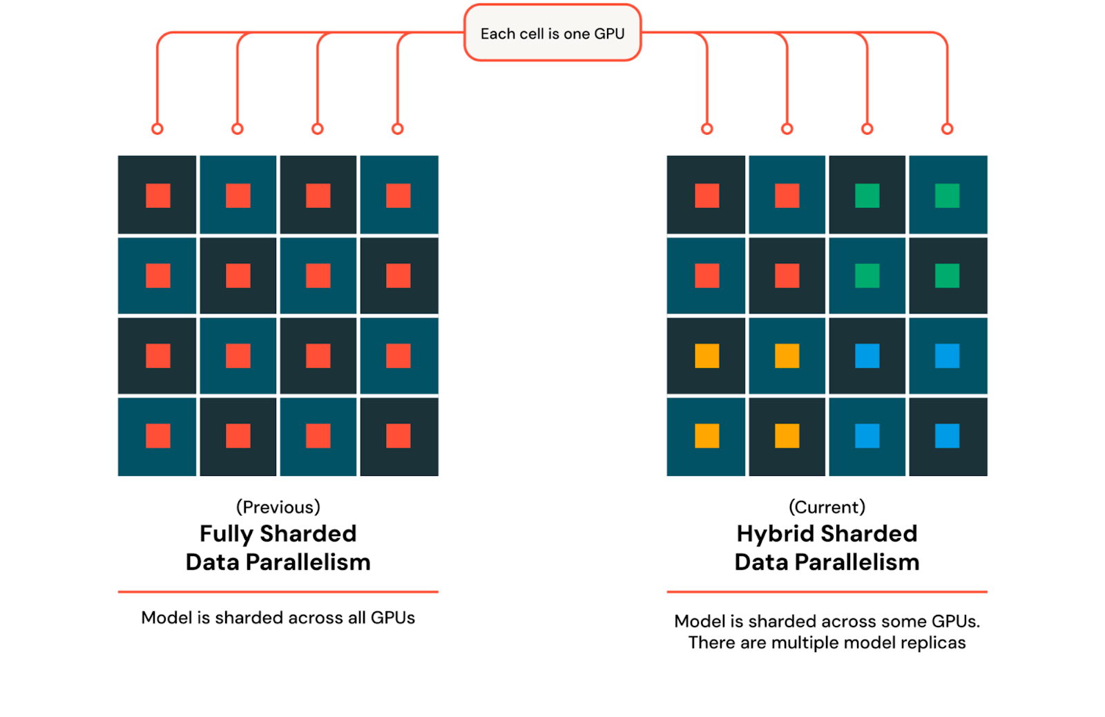
그림 4: FSDP와 HSDP / Figure 4: FSDP and HSDP

PyTorch를 사용하면 이 두 가지 유형의 병렬화를 효과적으로 결합하여, 전문가 병렬화와 같은 변형(something custom)을 구현할 때 저수준의 DTensor 추상화를 사용하면서도 FSDP의 더 고수준의 API를 활용할 수 있습니다. 이렇게 전문가 병렬화 샤드 차원과 ZeRO-3 샤드 차원, 그리고 순수 데이터 병렬화를 위한 복제 차원으로 구성된 3D 디바이스 메시를 구축할 수 있습니다. 이러한 기법들을 결합하여 매우 큰 클러스터에서 거의 선형적인 확장을 실현할 수 있으며, MFU 수치 40% 이상을 달성할 수 있게 됩니다.

With PyTorch, we can effectively combine these two types of parallelism, leveraging FSDP’s higher level API while using the lower-level DTensor abstraction when we want to implement something custom like expert parallelism. We now have a 3D device mesh with expert parallel shard dimension, ZeRO-3 shard dimension, and a replicate dimension for pure data parallelism. Together, these techniques deliver near linear scaling across very large clusters, allowing us to achieve MFU numbers over 40%.

Torch Distributed를 사용한 탄력적인 체크포인팅 / Elastic Checkpointing with Torch Distributed

내결함성(fault tolerance)는 특히 노드 장애가 일반적으로 발생할 수 있는 분산 환경에서 장기간(extended period)에 걸쳐 LLM을 안정적으로 학습시키는데 매우 중요합니다. 작업 중 불가피한 장애가 발생했을 때 진행 상황을 잃지 않기 위해, 매개변수와 옵티마이저 상태, 그리고 다른 필요한 메타데이터를 포함한 모델의 상태를 저장(checkpoint)합니다. 장애가 발생하는 경우, 시스템은 처음부터 다시 시작하지 않고 마지막으로 저장했던 상태에서 다시 시작할 수 있습니다. 장애 시의 견고성(robustness)를 보장하기 위해, 중단 시간(downtime)을 최소화할 수 있는 가장 성능이 좋은 방법으로 체크포인트를 자주 확인하고 저장 및 불러오기를 해야 합니다. 또한, 너무 많은 GPU들에서 장애가 발생하게 되면 클러스터의 크기가 변할 수 있으므로, 다른 수의 GPU에서 탄력적으로 다시 시작할 수 있는 기능이 필요합니다.

Fault tolerance is crucial for ensuring that LLMs can be trained reliably over extended periods, especially in distributed environments where node failures are common. To avoid losing progress when jobs inevitably encounter failures, we checkpoint the state of the model, which includes parameters, optimizer states, and other necessary metadata. When a failure occurs, the system can resume from the last saved state rather than starting over. To ensure robustness to failures, we need to checkpoint often and save and load checkpoints in the most performant way possible to minimize downtime. Additionally, if too many GPUs fail, our cluster size may change. Accordingly, we need the ability to elastically resume on a different number of GPUs.

파이토치(PyTorch)는 다양한 클러스터 구성에서 체크포인트를 저장하고 불러오기 위한 기능(utility)들을 포함하고 있는 분산 학습 프레임워크를 통해 탄력적인 체크포인팅 기능을 지원합니다. 파이토치 분산 체크포인트(PyTorch Distributed Checkpoint)는 노드 장애나 추가로 인한 클러스터 구성이 변경되는 것과 관계없이, 모델의 상태를 학습 클러스터의 모든 노드에서 정확하게 저장하고 복원할 수 있도록 합니다.

PyTorch supports elastic checkpointing through its distributed training framework, which includes utilities for both saving and loading checkpoints across different cluster configurations. PyTorch Distributed Checkpoint ensures the model’s state can be saved and restored accurately across all nodes in the training cluster in parallel, regardless of any changes in the cluster’s composition due to node failures or additions.

또한 매우 큰 모델을 학습할 때, 체크포인트의 크기가 매우 커져서 체크포인트 업로드와 다운로드 시간이 매우 느려질 수 있습니다. 파이토치 분산 체크포인트(PyTorch Distributed Checkpoint)는 분산 체크포인트를 지원하여 각 GPU가 모델의 해당 부분만 저장하고 불러올 수 있도록 합니다. 분산된 체크포인트(sharded checkpoint)를 탄력적 학습(elastic training)과 결합하면 각 GPU는 메타데이터 파일을 읽어 재시작(resumption) 시에 어떠한 부분(shard)을 다운로드할지 결정할 수 있습니다. 메타데이터 파일에는 각 텐서의 어떤 부분이 어떤 샤드(shard)에 저장되어 있는지에 대한 정보가 포함되어 있습니다. 그러면 GPU는 모델의 해당 부분에 대한 샤드를 다운로드하고 체크포인트의 그 부분을 불러올 수 있습니다.

Additionally, when training very large models, the size of checkpoints may be very large, leading to very slow checkpoint upload and download times. PyTorch Distributed Checkpoint supports sharded checkpoints, which enables each GPU to save and load only its portion of the model. When combining sharded checkpointing with elastic training, each GPU reads the metadata file to determine which shards to download on resumption. The metadata file contains information on what parts of each tensor are stored in each shard. The GPU can then download the shards for its part of the model and load that part of the checkpoint.

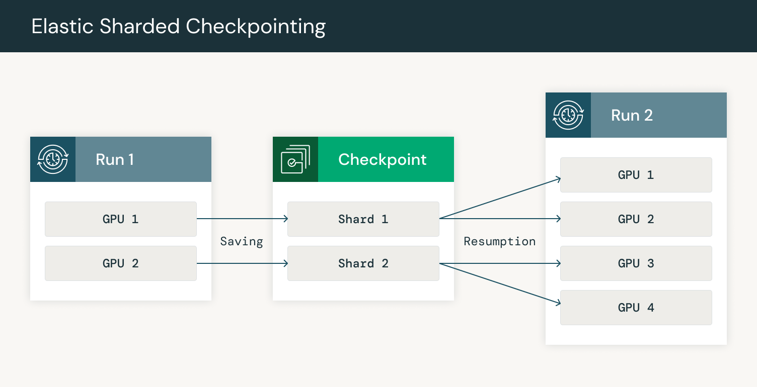
그림 5: 체크포인트 저장하고 추가된 GPU들에서 재개하기 / Figure 5: Checkpointing saving and resumption resharded on additional GPUs

GPU들 간의 체크포인트를 병렬화함으로써 네트워크 부하를 분산시키고 견고성(robustness)과 속도를 향상시킬 수 있습니다. 3000개 이상의 GPU를 사용하여 모델을 학습할 때, 네트워크 대역폭(bandwidth)이 빠르게 병목(bottleneck)이 됩니다. 우리는 먼저 한 복제(replica)에서 체크포인트를 다운로드한 다음, 다른 복제본들에 필요한 부분(shard)들을 보내는 식으로 HSDP의 복제 기능을 활용합니다. Composer와의 통합을 통해 30분 간격으로 체크포인트를 클라우드 저장소에 안정적으로 업로드하고, 노드 장애 발생 시 자동으로 최신 체크포인트로부터 5분 이내로 재개(resume)할 수 있게 됩니다.

By parallelizing checkpointing across GPUs, we can spread out network load, improving robustness and speed. When training a model with 3000+ GPUs, network bandwidth quickly becomes a bottleneck. We take advantage of the replication in HSDP to first download checkpoints on one replica and then send the necessary shards to other replicas. With our integration in Composer, we can reliably upload checkpoints to cloud storage as frequently as every 30 minutes and automatically resume from the latest checkpoint in the event of a node failure in less than 5 minutes.

결론 / Conclusion

파이토치(PyTorch)가 뛰어난 성능으로 최첨단(state-of-the-art) LLM을 학습할 수 있게된 것을 매우 기쁘게 생각합니다. 이번 글에서는 PyTorch Distributed와 MegaBlocks on Foundry를 사용하여 효율적으로 전문가 혼합(MoE) 학습을 구현하는 방법을 보여드렸습니다. 또한, 파이토치(PyTorch) 탄력적 체크포인팅(Elastic Checkpointing)을 사용하여 노드 장애 발생 시 다른 수의 GPU에서 빠르게 학습을 재개할 수 있었습니다. PyTorch HSDP를 사용하여 학습을 효율적으로 확장하고 체크포인트 재개 시간을 개선할 수 있었습니다. 우리는 강력하고 활기찬 오픈소스 커뮤니티를 통해 훌륭한 AI 모델을 모두에게 제공할 수 있기를 기대합니다. LLM Foundry와 PyTorch 저장소를 방문하여 훌륭한 모델을 구축하는데 동참해주세요.

We’re very excited to see how PyTorch is enabling training state-of-the-art LLMs with great performance. In our post, we’ve shown how we implemented efficient MoE training through PyTorch Distributed and MegaBlocks on Foundry. Furthermore, PyTorch elastic checkpointing allowed us to quickly resume training on a different number of GPUs when node failures occurred. Using PyTorch HSDP has allowed us to scale training efficiently as well as improve checkpointing resumption times. We look forward to continuing building on a strong and vibrant open-source community to help bring great AI models to everyone. Come join us in building great models at LLM Foundry and PyTorch.